Managing Complexity and Technical Debt : A Model for Quantifying Systemic Analysis

1. Introduction

Today’s post is a summer recreation/musing about how to model the effect of complexity and technical debt, in the same spirit of a the previous “Sustainable IT Budget in an equation” post. I used the word “recreation” to make it clear that this is proposed as “food for thoughts”, because I have worked hard to make the underlying model really simple, without the intent of accuracy. I have worked on IT cost modelling since 1998 and have removed layers of complexity and precision over the years to make this model a communication tool. You may see the result, for instance, in my lecture at Polytechnique about IT costs.

This post is a companion to the previous “Sustainable Information Systems and Technical Debt” with a few (simple) equations that may be used to explain the concepts of sustainable development  and complexity management to an audience who loves figures and quantified reasoning. It proposes a very crude model, that should be used to explain the systemic behavior of IT costs. It is not meant to be used for forecasting.

What is new in this model and in this post, is the introduction of change and the cumulated effect of complexity. The previous models looked at the dynamics of IT costs assuming an environment that was more or less constant, which is very far from the truth, especially in a digital world. Therefore, I have extended this simple model of IT costs into two directions:

• I have introduced a concept of « decay » to represent the imperative for change. I am assuming that the value delivered by an IT system decreases over time following a classical law of “exponential decay”. This is a simple way to represent the need for « homeostasis », which is the need to keep in synch with the enterprise’s environment. The parameter for decay can be adjusted to represent the speed at which the external environment evolves.
• I have also factored the effect of cumulated complexity into the model, as a first and simple attempt to model technical debt. This requires modelling the natural and incremental rise of complexity when IS evolves to adapt to its environment (cf. previous point) – as noticed before, there is a deep link between the rate of change and the importance of technical debt – as well as the representation of the effort to clean this technical debt.

This model makes use of Euclidean Scalar Complexity(ESC), a metric developed with Daniel Krob and Sylvain Perronet to assess integration complexity from enterprise architecture schema. ESC is easy to compute and is (more or less) independent from scale.  The technical contribution of this new model and blog post is to propose a link between ESC and technical debt. Although this link is somehow naïve, it supports “business case reasoning” (i.e., quantifying common sense) to show that managing technical debt has a positive long-term return on investment.

This post is organized as follows. Section 2 gives a short summary of asset management applied to information systems, in other words, how to manage information systems through replacement and renovation rates. This is the first systemic lesson: investments produce assets that accumulate and running costs follow this accumulation. The proposed consequence is to keep the growth and the age of the assets under control. Section 3 introduces the effect on computing (hardware) resource management on IT costs. We make a crude distinction between legacy systems where hardware is tied to application in a way that required a complete application re-engineering to benefit from better generations of computing resources, as opposed to modern virtualized architecture (such as cloud computing) that supports the constant and (almost) painless improvement of these resources. This section is a simplified application of the hosting cost model proposed in my second book, which yields similar results, namely that Moore’s law benefits only show in IT costs if the applicative architecture makes it possible. Section 4 introduces the need for change and the concept of exponential decay. It shows why managing IT today should be heavily focused on average application age, refresh rate and software asset inertia. It also provides quantitative support for concepts such as multi-modal Information Systems and Exponential Information Systems. Section 5 is more technical since we introduce Information System complexity and the management of technical debt from a quantified perspective. The main contribution is to propose a crude model about how complexity increases iteratively as the information system evolves and how this complexity may be constrained through refactoring efforts at the enterprise architecture level. Although this is a naïve model, at a macro scale, of technical debt, it supports quantified reasoning which is illustrated throughout this blog post with charts produced with a spreadsheet.

2. Asset Management and Information Systems

We will introduce the model step by step, starting with the simple foundation of asset management. At its simplest, an information system is a set of software assets that are maintained and renewed. The software process here is very straightforward: a software asset is acquired and integrated into the information systems. Then it generates value and costs: hosting costs for the required computing assets, support costs and licensing costs. The previously mentioned book gives much more details about the software assets TCO; this structure is also found in Volle  or Keen . The software lifecycle is made of acquisition, maintenance, renewal or kill.

Since the main object of the model is the set of software assets, the key metric is the size of this asset portfolio. In this example we use the Discounted Acquisition Costs model, that is the sum of the payments made for the software assets that are in use (that have not been killed) across the information system’s history.  The IS budget has a straightforward structure : we separate the build costs (related to the changes in the asset portfolio : acquisition, maintenance, etc.) and the run costs (hosting, support and licensing). Run costs are expressed directly as the product of resource units (i.e. the size of the IS / software assets) and unit costs (these unit costs are easy to find and to benchmark).

The model for the Build costs is more elaborate since it reflects the IS strategy and the software product lifecycle.  To keep things as simple as possible we postulate that the information system strategy in this model is described as an asset management policy, with the following (input) parameters to the model:

• The total IT budget
• The percentage of Build budget that is spent on acquiring new assets (N%)
• The percentage of Build budget that is spent on retiring old assets (K%)
• The percentage of Build budget that is spent on renewals (R%)

With these four parameters, the computation of each yearly iteration of the IT budget is straightforward. The run costs are first obtained from the IS size of the previous year. The build budget is the difference between total IT budget and run costs. This build budget is separated into four categories: acquiring new assets, killing existing (old) assets, replacing old assets with newer ones (we add to the model an efficiency factor which means that renewals are slightly more efficient than adding a brand-new piece of software) and “maintenance”. Maintenance (for functional or technical reasons) is known to produce incremental growth (more-or-less, it depends on the type of software development methodology) which we can also model with a parameter.

The model is, therefore, defined through two key equations which tells how the asset portfolio changes every year in size (S)  and age (A). Here is a simplified description (S’ is the new value of “assets size”, S is the value for the previous year):

1. Growth of the assets:  S’ =  S -  Build x K% + Build x A% + Build x (1 – K% – A% – R%) x G%
2. Ageing of the assets:  A’ = (A + 1) x (S – Build * (1 – N% - R% - K%)) / S’

Measuring software assets with Discounted Acquisition Costs has benefits and drawbacks. The obvious benefit is that it is applicable to almost all companies. The value that is used for discounting with age has a small effect on the overall simulation (and what will be said in the rest of the post). Typical values are between -3% to -10%. The drawback is that money is a poor measure of complexity and richness of the software assets. A better alternative is to use function points, but this requires a fair amount of efforts, over a long period of time. When I was CIO of Bouygues Telecom, I was a strong proponent of function points but I found it very hard to make sure that measurement was kept simple (at a macro scale) to avoid all the pitfalls of tedious and arguable accounting. What I have found over the years is that it is almost impossible to use function points without strong biases. However, as soon as you have a reasonable history, it works very well for year-by-year comparisons. Used at a macro scale, it also gives good benchmarking “orders of magnitudes”.  There are many other alternatives (counting apps, databases, UI screens, ….) that suffers from the same benefits and drawbacks. Since I aim to propose something generic here – and because discussing with CFOs is a critical goal of such a model -, using DAC makes the most sense.

The following chart gives an example of simulating the same information system, with the same constant budget, under three strategies:

• The “standard strategy” is defined by N% = 5%, K% = 3%, R% = 50%. With 50% of the project budget spent on renewal, this is already a strong effort to keep the assets under control. The imbalance between what needs to be added (5% of the budget to meet new needs and a small effort for decommissioning) is quite typical.
• The “clean strategy” is defined by N% = 5%, K% = 8%, R%=60%. Here we see the effect of try to clean up the legacy (more renewal effort, and more decommissioning).
• The “careless” scenario is defined by N% = 5%, K% = 3% and R% = 30%. This is not a large change compared to the standard one, less effort is made on renewing assets so that more money can be spent on adapting the existing assets to the current needs.

These three figures illustrate some of the key lessons that have been explained before, so I will keep them short:

• Changes that may seem small in the strategy (the values from the three scenarios are not all that different) produce significant differences over the years. Especially the “Build/Run” ratio changes significantly here according to the strategy that is picked.
• Beware of accumulation, both in size and ageing, because once the problem accumulates it becomes hard to solve without a significant IT budget increase.
• The effects of an aggressive cleanup asset management strategy are visible, and pay for themselves (i.e., they help free build money to seize new opportunities), but only after a significant period of time, because of the multiplicative effects. Therefore, there is no short-term business case for such a strategy (which is true for most asset management strategies, from real estates to wine cellars).

As I will explain in the conclusion, showing three examples does not do justice to the modelling effort. It is not meant to produce static trajectories, but rather to be played with in a “what if” game. Besides, there are many hypotheses that are specific to this example:

• The ratio between the Build budget and the value of the asset portfolio is critical. This reflects the history of the company and differentiates between companies that have kept their software assets under control and those where the portfolio is too large compared to the yearly budget, because accumulation has already happened.
• This example is built with a flat budget, but the difference gets bigger if there are budget constraints (additional project money is “free money” whereas “less project money” may translate to forced budget increase because renewing the SW assets is mandatory for regulatory reasons … or because of the competition).
• The constants that I have used for unit costs are “plausible orders of magnitudes” gathered from previous instances of running such models with real data, but each company is different, and the numbers do change the overall story.
• We do not have enough information here to discuss about the “business case” or the “return on investment” for the “cleanup strategy”. It really depends on the value that is generated by IT and the “refresh rate” constraints of the environment, which is what we will address in Section 4.

3. Managing Computing Infrastructures to Benefit Moore’s Law

In the previous model I have assumed that there is a constant (cf. the unit cost principle) cost of hosting a unit of software asset on computing resources. This is an oversimplification since hosting costs obviously depends on many factors such as quality of service, performance requirement and software complexity. However, when averaged over one or many data centers, these unit costs tend to be pretty “regular” and effective to forecast the evolution of hosting. There is one major difference that is worth modelling: the ability to change, or not, the computing & storage hardware without changing the software asset. As explained in my second book,  “Moore’s Law only shows in IT costs if it is leveraged”, that is if you take advantage of the constant improvement of hosting costs. To keep with the spirit of a minimal model, we are going to distinguish two types of software:

• Legacy: when the storage/computing configuration is linked to the application and is not usually changed until a renewal (cf. previous section) occurs. In this case, unit costs tend to show a slow decline over the years, due to automation and better maturity in operation, which is very small compared to the cost decrease of computing hardware. This was the most common case 20 years ago and is still quite frequent in most large companies.
• Virtualized: when a “virtualization layer” (from VM, virtual storage to containers) allows a separation between software and computing assets. This is more common nowadays with cloud (public or private) architecture. Because it is easier to shift computing loads from one machine to another, hosting costs are declining more rapidly. This decline is much slower than Moore’s law because companies (or cloud providers) need to amortize their previous investments.

This split is easy to add into our asset model. It first requires to track software assets with two lines instead of one (legacy and virtualized), and to create two set of unit costs (which will reflect the faster reduction for virtualized hosting cost, as well as the current difference which is significant for most companies since virtualized load tend to run on “commodity hardware” whereas legacy software often runs on specialized and expensive hardware (the most obvious example being the mainframe).

The software asset lifecycles are coupled as follows. First the kill ratio K% must be supplemented with a new parameter that says how much of the effort is made on the legacy portfolio compared to the virtualized one. Second, we assume here – for simplification – that all applications that are renewed are ported to a newer architecture leveraging virtualized computing resources. Hence the renewal parameter (R%) will be the main driver to “modernize” the asset portfolio.

The following curves show the difference between three strategies, similarly to the previous section. We have taken a generic example where the portfolio is balanced at first between legacy and virtualized computing architecture. In this run, the new ratio (N%) is raised to 10% to reflect a situation where more change is required. The difference is mostly about the renewal rate (respectively 40%, 50% and 30%) and the kill rate (respectively 3%, 5% and 3%). The figure shows the size of the two software asset portfolios (Virtualized and Legacy) as well as the average age.

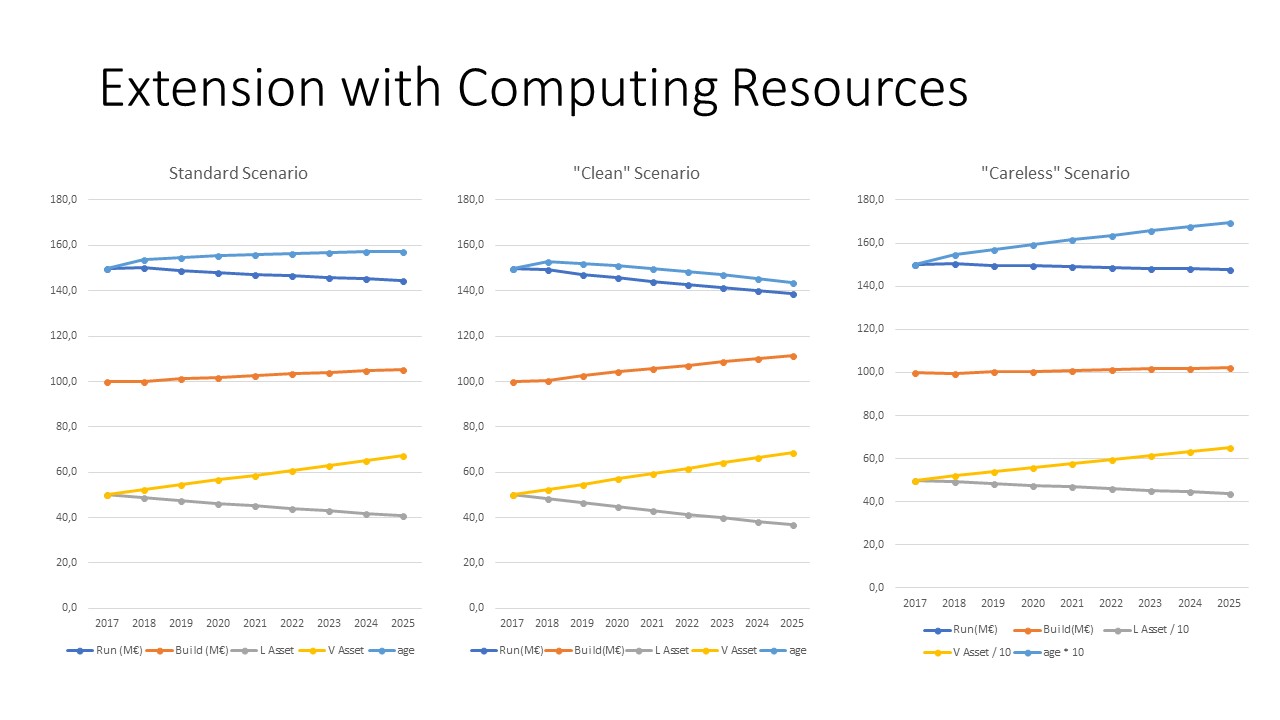
The model was run here with conservative costs estimates on purpose. The reader is encouraged to run this type of computation with the real values of unit cost that s/he may observe in her company. Even with this conservative setting, the differences are quite significant:

• A sustained renewal effort translates into a more modern portfolio (the difference in average age is qui significant after 8 years) and lower run costs. It is easy to model the true benefits of switching to commodity hardware and leveraging virtualization.
• The difference in the Build/Run ratio is quite high, because the run costs are much lower once a newer architecture is in place.
• These efforts take time. Once again, the key “strategic agility” ration is “build/run”. When the asset portfolio has become too large, the “margin for action” is quite low (the share of the build budget that can be freely assigned to cleanup or renewal once the most urgent business needs have been served).

To make these simulations easier to read and to understand, we have picked a “flat IT budget scenario”. It is quite interesting to run simulations where the “amount of build project” has a minimal value that is bound to business necessities (regulation or competition – as is often the case in the telecom market). With these simulations, the worse strategy translates into a higher total IT cost, and the gap increases over the years because of the compounded effects.

4. Managing Information Systems Refresh Rate to Achieve Homeostasis

I should apologize for this section title which is a mouthful bordering on pretentious … however I have often used the concept of “homeostasis” in the context of digital transformation because it is quite relevant. Homeostasis refer to the effort of a complex systems (for instance a living organism) to maintain an equilibrium with its environment. In our world of constant changes pushed by technology rapid evolution, homeostasis refers to the constant change of the information system (including all digital assets and platforms) to adapt to the changing needs of customers and partners. From my own experience as an IT professional for the past 30 years, this is the main change that has occurred in the past decade: the “refresh rate” of information systems has increased dramatically. This is an idea that I have developed in many posts from this blog.

This is also a key idea from Salim Ismail’s best seller book “Exponential Organizations” which I have used to coin the expression “Exponential Information Systems”. From our IT cost model perspective, what this says is that there is another reason – other than reducing costs and optimizing TCO – to increase the refresh rate. I can see two reasons that we can to capture: first, the value provided by a software asset declines over time because the environment changes. Second, no software asset is isolated any more, each is part of a service (or micro service) orchestration patterns, that comes with its own refresh rate constraints. I have found that the best way to express both principles is to postulate that the value provided by a software asset declines over time following a classical exponential decay law: 

                Value = V0 x exp(- lambda x time)

This formula is easy to introduce in our model, and it adds a penalty to ageing software that is independent from the previously mentioned TCO effects on licensing, maintenance, or hosting.  The decay parameter (lambda) is a way to tell the model that “software must change regularly” to cope with the constant changes of its environment.

I will not offer any simulation or charts here, because it is actually quite difficult to find data about this “decay” (need for change) and it makes little sense to invent one for a generic simulation. Also, not all software assets are equal with respect to exponential decay. Software-as-a-service (SaaS) is precisely an answer to this need for constant adaptation. Therefore, should we plan to run simulations seriously, we should use different decay constants for different classes of assets. There are plenty of software costs benchmarking materials that may be used to calibrate or evaluate the unit costs for the two previous models but evaluating the “rate of decay” is much more difficult and very specific to each industry.

On the other hand, exponential decay / forced rate of change is a really useful concept when planning about the long-term future of information systems. When one plays with the previous model augmented with decay, it becomes clear that the desired rate of change, which is a business imperative, is not compatible with the inertia that is exhibited by the model. This should be clear in the example shown in the previous section: the weight of the legacy portfolio is too high to obtain a homogeneous high refresh rate. In most large and established company, the Build/Run ratio is worse that what is proposed here, which means that the ability to increase the refresh rate is even worse.

This situation yields naturally to the concept of “multi-modal IT”, including the famous “bimodal IT” pattern.  A multi-modal information system is organized in an “onion structure” with a core and layers towards the periphery. Using API (Application Programming Interfaces), the onion may be organized so that the refresh rate is higher in the outside layers than in the core. This a direct application from biology and a pattern that is used in many organization theories such as betacodex. This is also the foundation for Exponential Information Systems: Use Enterprise Architecture and modularity to support different refresh rates for different parts of the information systems. The core/shared/pivot/common data model, that described the key business objects that are used throughout the multiple layers (multi-modal component) is a critical component of the Enterprise Architecture since it defines the agility through the API. A modular multimodal architecture is one that leaves most of the changes in the layers that were designed to accommodate high refresh rates. This means that modularity is a dynamic property of system architecture much more than a static one.

The lesson from this short section is that one should think really hard about the required refresh rates of sections of their information systems. For each functional domain, a target refresh rate (which is equivalent to a target average age for software assets) should be set. This target is both a business and technical imperative which should be based on requirements from customers and partners, as well as constraints related to software ecosystems. Many software environments, such as developing a mobile application, come with their own refresh rate constraints because the key features provided by the ecosystem change constantly … while upward compatibility is approximate at best. Similarly, the ambition to leverage artificial intelligence and machine learning for a given business domain should translate into setting a high refresh rate target. Keep in mind that adapting to the outside environment is a business imperative: if the lack of architecture modularity and the inertial of the accumulated weight of the asset portfolio prevent from upgrading the portfolio fast enough, the obvious solution is to grow this portfolio resulting in added complexity and IT costs.

5. Information Systems Complexity and Technical Debt

This last section introduces complexity and its effect on TCO in our IT cost model. We have seen throughout this post that the accumulation of weight is a burden, we shall now see that the accumulation of complexity is also a handicap that translates into additional costs, namely integration, testing and support costs. Obviously, the complexity of information systems reflects the complexity of their mission and the complexity of their environment. Somehow, this complexity is where part of the business value and differentiation is created. What we want to focus on here is the excess of complexity, which is precisely the definition of technical debt.

To introduce complexity in our model, we need a way to define and measure it. We shall use “Euclidean Scalar Complexity” because it is easy to understand and has a set of unique properties that makes it the best candidate for managing complexity at the Enterprise Architecture scale. The principle is quite simple. Assume that you have an architecture schema of your information systems, with boxes and links. Assume that you have a weight w(b) for each of the boxes, and that the existence of a link on your schema represents an interaction between the two subsystems represented by the box.  The weight could be the DAC measure of Section 2, the function points, or any additive metric that you like (i.e. w(a+b) = w(a) + w(b)). The Euclidean Scalar Complexity (ESC) of your architecture (abstraction of your system) is the square root of the sum of:  w(x) x w(y) for all pairs of boxes x, y that are either identical or joined with a link on the architecture schema. Normalized ESC means dividing the ESC value by the weight of the information systems, which yields a complexity ratio that we shall use in our model, a number between 0 and 1 (1 means that everything is connected and a value close to zero means that every piece is independent).

ESC is one of the few metrics that is “scale invariant”, which is the first requirement for working at the whole IS schema (each architecture schema is a crude abstraction) – see the 2007 paper “Complexité des systèmes d’information: une famille de mesures de la complexité scalaire d’un schéma d’architecture” by  CASEAU Y., KROB D., PEYRONNET S. Being scale invariant means that if a change of scale is applied to the representation (more boxes and more links to represent the same information at a different scale), the complexity does not change. Another short introduction to ESC is provided in my Polytechnique lecture. There is no need to understand ESC in detail to see how it can be used to extend our IT cost model to manage technical debt, but the key insight that can help is to see that ESC is foremost a (static) modularity measure. ESC works well because it captures the benefits of Enterprise Architecture patterns such as gateways, integration buses, API encapsulation, etc. ESC is a great metric to capture the complexity of micro-service architectures.

As explained earlier, we do not suppose that the ideal information system has no complexity, but rather that for a given set of assets, there exists two complexity ratios, Cmin and Cmax, that represent on the one hand the minimal achievable ESC (i.e. rebuilding the IS from zero using the maximal possible modularity) and on the other hand, the complexity that one would get by randomly adding and integrating software assets incrementally. We used the normalized ESC, so these two numbers are between 0 and 1. Not all architecture problems are equal: some information systems are easy to build which translates into Cmin and Cmax being close. On the other hand, for many systems, the difference between Cmin, Cmax and C (the actual ESC ratio) is quite high. These two anchors makes possible the definition of technical debt as: w(S) x (C – Cmin) / (Cmax – Cmin)

Introducing technical debt into our cost model means two things:

• Measuring the impact of this additional complexity on costs.
• Defining and measuring what “reducing the technical debt” (i.e., managing complexity) may mean, in terms of effect and cost.

The first part is easy, considering the simplicity of our model and the fact we are just looking for simple orders of magnitude. In a same way that we have take the effect of aging into account for licensing, we upgrade the following formulas:

• Integration costs are proportional to the ESC : for a project with no complexity at all it would be zero (negligible compared to the cost of building / buying the new component) whereas for a truly complex (C = 1.0) system, integration (and testing) costs are equal to the acquisition costs. This is very debatable (because it is so simple and because integration costs may be even worse) but it gives a first plausible value.
• Support costs are also impacted: a fraction of support costs is proportional to C. This fraction is different for each information systems and depends on the nature of support activities (for instance, level 1 support is less impacted than level 3 support). Thus, this fraction is left as a model parameter.

The second part is the true extension of the model and what makes this post a new contribution to IT cost modelling.  

• Complexity without any refactoring effort evolves naturally towards Cmax as an asymptotic value (which is the definition of Cmax). The speed of evolution depends on how much of the information system is renewed each year, so the resulting complexity is a weighted average of the previous one and Cmax, where the weights are respectively the size of what is untouched in the portfolio and the size of what is added.
• Refactoring is seen as a fraction of the renewal budget applied to reducing the complexity. The effect is described by a power law (declining return of the invested money). The maximal effect (the asymptotic value) is getting the complexity to Cmin (also by construction). I have used a power law with degree 4 which seems to reproduce the empiric observation that the refactoring efforts have a law of strongly diminishing returns (the last 60% benefits cost 80% of the effort).

The following illustration compares three IT strategies while taking technical debt into account. In this example we assume Cmin = 0.3 and Cmax = 0.6, with C = 0.5 at present time. The new parameters compared to section 1 are the amount of refactoring (F%) and how much of the kill effort is targeted towards legacy (small effect since the kill effort is small here).

1. The “standard strategy” is defined by N% = 5%, K% = 3%, R% = 40% and F%=15%. Here 40% of the project budget is spent on renewal, and 15% of that money is reserved for refactoring. 70% of the kill effort is targeted towards legacy. The ESC ratio evolves from 0.5 to 0.489.
2. The “intense strategy” is defined by N% = 5%, K% = 5%, R%=50% and F= 30% with 80% of kill effort put on legacy. This is a more sustained effort (since money applied to refactoring is not applied to adding new software assets). The complexity ration evolves from 0.5 to 0.464.
3. The “careless” scenario is defined by N% = 5%, K% = 3% and R% = 30% and clean = 5%. These values are quite representative of most IT strategies (cf. what we said earlier, 30% of renewal is already the sign of a managed portfolio, many companies suffer from worse accumulation). Here the complexity moves from 0.5 to 0.509

These simulations are only proposed as an illustration. What can be learned through repeated simulations is similar to what we said in Section 2:

• Efforts to clean up the portfolio, to keep the age and the complexity under control, are long-term efforts but they have lasting effects.
• Accumulation in complexity, as well as accumulation in weight, has the dual effect of increasing the run costs and reducing the agility (the effort to change the information system to add new capacities becomes higher).
• Contrary to section 2 and 3 where the models may be calibrated with well-known unit costs, measuring the negative effect of complexity and the positive effect of refactoring is hard. What is proposed here is a simple and conservative model that has the benefit of showcasing the effects of both but finding the right constant /parameters to match this model to your reality requires efforts and will lead to some “guesstimates”.
• The key benefit of keeping weight and complexity under control is to allow for a higher refresh rate, which is itself a business imperative which can be modelled through “value decay” (Section 4). In order to simulate the value created by an aggressive “keep the complexity under control” strategy, you need to work under the situation of strong need for refresh (high decay). The weight of technical debt becomes a huge burden as soon as the environment requires to constantly update the information system.

6. Conclusion

The title for this blog post is: “Managing Complexity and Technical Debt: A Model for Quantifying Systemic Analysis”. There are two key ideas  here : the first one is “quantifying” and the second one is “systemic”. Both are related to the fact that this proposed model is foremost a communication tool. I decided to build a quantified model because this is the best way to communication with business managers. It does not mean that this model should be used for forecasting future IT costs, it is by far to simplistic. Using models and simulation is a great way to communicate with CFOs; they are even more effective if they rely on simple parameters/KPI such as unit costs that can be evaluated through benchmarking (cf. the Gartner paper on how CIOs can work with CFOs). To make this communication tool work for your case requires using your own data, as was said repeatedly.

The second benefit of working with a model is the benefit of simulation, which is a free benefit once you have built your own spreadsheet. Being able to play “what if” scenarios is critical to help your stakeholders understand the systemic nature of the IT costs:

• Delays: good decisions may have long delays before showing their positive consequences
• Accumulation: this is the main difficulty of managing information systems, once the cost problems are visible, they are much harder to solve.
• Amplification (reinforcement): bad decisions produce waste that adds to the complexity and the overall weight, producing further problems along the way.

Although the topic is very different from the topics that I have covered using GTES (Game Theoretical Evolutionary Simulation), one can find the same pattern : a simple model is used to create simulations that are organized into a serious game from which systemic insights may be gained. As was stated earlier, the goal here is not to define the “best IT asset management strategy” using a crude model, but to gain a systemic understanding why long-term complexity-constrained asset management policies must be implemented.

Here are the conclusions that I can draw from playing with this generic model (more detailed conclusions would require working a on a specific instance):

1. Keep the age of your software assets under control
2. Keep the scope as small as possible (but not smaller, to paraphrase Einstein)
3.  Constantly refactor your information systems, at different scales.